SITCOMTN-137

Getting Started with Cell-Based Coadds

This is a draft.

By:

• Miranda R. Gorsuch
• Arun Kannawadi

Abstract

As development for cell-based coadds continue, their testing will become pertinent during the commissioning process. This technote is meant to be an initial guide to generating and using cell-based coadds within the context of the LSST Science Pipelines and USDF, where several example use cases will be outlined in the form of brief code snippets and initial analyses. Example code will also be maintained in the form of Jupyter notebooks, currently found here.

How to generate cell-based coadds

Generating cell-based coadds requires some familiarity with the LSST Science Pipelines and butler repositories. This section will focus on the details that are relevant to this specific use-case. Further documentation for using the pipelines can be found here.

Setup at USDF

You will need to setup a pipelines stack, which is updated regularly. To pick out the latest weekly update, run source /sdf/group/rubin/sw/w_latest/loadLSST.bash. This is a common choice for the sake of stability, though specific daily releases are also available, for example source /sdf/group/rubin/sw/tag/d_2024_08_27/loadLSST.bash. Once you have sourced your favorite bash file, run setup lsst_distrib to start using your environment.

Occasionally, it might be useful to have a different version of a package within the current stack, especially in the case of ticket branches. A good troubleshooting tip will be to run eups list -s | grep ${USER}, which will list all locally setup packages.

Running the pipetask command

The pipetask run command is what will generate the coadds. This command will be run in the context of a specific butler repository. The /sdf/data/rubin/repo/main repo is a good example. Generating cell-based coadds as done in this technote follow the format of the snippet below:

pipetask run -j 4 --register-dataset-types \
-b /sdf/data/rubin/repo/main \
-i HSC/runs/RC2_subset/d_2024_08_27 \
-o u/$USER/cell_coadds \
-p /sdf/group/rubin/user/mgorsuch/cell-coadd/pipeline.yaml \
-d "instrument='HSC' AND skymap='hsc_rings_cells_v1' AND tract=9813 AND band='i'"

The pipetask run command requires the following components:

• -b

  • This defines which butler to use. Here, it’s easiest to use the one already defined within the main repository.

• -i

  • This defines the input collection. Note that it’s good practice to generate and use the coadds on the same daily stack as the original run. For instance, it’s best to use the d_2024_08_27 daily stack environment when using the HSC run from d_2024_08_27. While it’s possible to run the coadds on a mismatching stack, this is good way to avoid possible inconsistencies.

• -o

  • This is the output collection. The output collection is stored in /sdf/data/rubin/repo/main/u/$USER/cell_coadds. The $USER term is useful to as to not accidentally save the output collection in a different user folder.

• -p

  • This is where the pipeline file is stored. This will define which tasks to run, and with what specific configurations. A bare-bones pipeline file is shown below.

• -d

  • The dataset query. This is for limiting the data with whatever is specified. Useful for either specific investigations or reducing the time for the command to run.

An example pipeline.yaml file:

description: A simple pipeline to test development of cell-based coadds.
 
tasks:
    makeDirectWarp: 
        class: lsst.pipe.tasks.make_direct_warp.MakeDirectWarpTask
        config:
            doWarpMaskedFraction : true
            doPreWarpInterpolation : true
    assembleCellCoadd:
        class: lsst.drp.tasks.assemble_cell_coadd.AssembleCellCoaddTask

With this pipeline, there are two tasks defined: makeDirectWarp and assembleCellCoadd. The warping task is not necessarily constrained to cell-based coadds, but is not run by default in the HSC runs we’re accessing, so it must be specified. The tasks also contain information on the required input data types, which are accessed from the input collection defined in the pipeline run command. This is extremely helpful to avoid rerunning all tasks prior to the coaddition state, though only in the case where all defaults prior to coaddition can be kept.

While most of the default config settings are sufficient, there are a few overrides that are necessary in the warping task for generating the mask fraction plane. The first config, doWarpMaskedFraction, is needed to generate the actual mask fraction object. However, the second config, doPreWarpInterpolation, will trigger the actual warping of the mask plane (BAD, SAT, and CR masks by default) that produces the mask fractions. Without this second config setting, the mask fraction plane will contain only 0 and NaN values.

One helpful command component is -c, which is used to override configs. The general format is -c <task name>:<config name>=<value>. For an example, let’s say the above pipetask command was run, but another run is necessary to test what happens if calc_error_from_input_variance is set to false. There’s no need to rewrite the original pipeline.yaml file; rather, this can be achieved with the pipetask command by adding a line -c assembleCellCoadd:calc_error_from_input_variance=False.

pipetask Outputs

The example pipetask command will generate several useful data structures within the output collection.

• deepCoadd_directWarp

  • An object of this type will contain the warped calexp image (or just warp) of a specific visit. Contains components like the image, mask, and variance planes of the warp, as well as PSF information.

• deepCoadd_directWarp_noise{n}

  • A noise realization generated from the variance plane of the input calexp. The default config setting calculates the median of the variance plane and then samples from a Gaussian distribution with a variance equal to the median value. Multiple noise planes can be generated for each warp, hence the {n} notation.

• deepCoaddCell

  • The coadd object containing the cell information for a specified patch. Image, mask, and variance planes are specific to individual cells, though these planes can be accessed at the patch level by combining cells together to generate a “stitched” coadd.

• deepCoadd_directWarp_maskedFraction

  • This object stores the mask fraction associated with each pixel. Interpolated masks cannot be represented with binary values since they are “smeared” across neighboring pixels due to the warping process.

Sample Butler Commands

This section collects a few useful commands and snippets that can help maintain and keep track of collections using the butler.

Query user collections (should be run within your user directory): butler query-collections /repo/main u/${USER}/*

Remove collections from your user directory example (do this first before removing runs): butler remove-collections /sdf/group/rubin/repo/main u/${USER}/<collection name>

Remove orphaned runs (can also replace the wildcard with a specific run):  butler remove-runs /repo/main u/${USER}/<collection name>/*

Note that these commands don’t remove the folders containing the removed data. Once the collection and runs have been removed using the butler commands, the folder itself will be OK to remove using typical terminal commands.

Occasionally it will be necessary to remove a registered dataset type from the butler entirely (across all collections in the repository, so some caution is warranted!). This is typically due to structural changes during development. First, it will be useful to see which collections contain the dataset type to be removed. The easiest outcome will be when the only collections queried will be your own, but in the case it’s not, notify the owner(s) of collections which contain the dataset to be removed. To search for these collections, you can use the Python snippet below:

collections = registry.queryCollections()

refs = registry.queryDatasets('deepCoadd_directWarp_maskedFraction', collections = collections)

print(np.unique([ref.run for ref in refs]))

To then remove the dataset type, you use the following command: butler remove-dataset-type /repo/main "<dataType name>". The runs containing the removed dataset type will still need to be removed.

Common Coding Patterns & Algorithms

There are a few common snippets of code that are especially helpful when working with cell-based coadds and their data structures.

Butler in a Notebook

Analyses using coadds are commonly done in a Jupyter notebook environment, such as the Rubin Science Platform. Accessing the cell-based coadds generated from the pipeline commands is best done using a butler, which can be setup within the notebook by specifying a repository and a collection. Generally, this sequence will look like this:

REPO = '/sdf/data/rubin/repo/main/'

from lsst.daf.butler import Butler

butler = Butler(REPO)
registry = butler.registry

collection = '<path to collection>'

The collection will be the output collection defined in the pipetask command; in this case, that output collection would be u/$USER/cell_coadds/<run name> (replacing &USER with the appropriate username). The run name will encode the time the collection was generated and will have the format YYYYMMDDTHHMMSSZ.

Now objects from the butler can be called. For instance, this technote will refer to coadd and warp objects as the following objects (though the exact parameters may change):

coadd = butler.get('deepCoaddCell', 
                     collections=collection, 
                     instrument='HSC', 
                     skymap = 'hsc_rings_cells_v1', 
                     tract = 9813, 
                     patch=61,
                     band='i',)

warp = butler.get('deepCoadd_directWarp',
                   collections = collection,
                   instrument='HSC',
                   skymap = 'hsc_rings_cells_v1',
                   tract = 9813,
                   patch = 61,
                   visit = 30482)

Iterating over Cells

The most common tool in using cell-based coadds is the iteration over a collection of many cells to collect their information in an organized manner. Currently, there are two main approaches.

The first is straight-forward, and is simply requires calling list(coadd.cells.keys()). This will provide a list of Index2D objects for all filled cell indices, skipping over empty cells. While iterating over this list, the information of the cell can be called with the Index2D object using coadd.cells[Index2D].

The second method is for displaying information in a grid format, such as a 2D histogram of cell values. The list in the first method will need to be expanded to include the empty cells that were initially skipped over. To achieve this, two lists are used: cell_list and cells_filled. The cell_list object is meant to store all possible iterations of Index2D objects, while cells_filled keeps tracks of which indices within cell_list are actually filled.

cell_list_filled = list(coadd.cells.keys())
cell_list = []
cells_filled = [False] * coadd.grid.shape[0] * coadd.grid.shape[1]

index = 0
for i in range(coadd.grid.shape[1]):
    for j in range(coadd.grid.shape[0]):
        cell_list.append(Index2D(x=j,y=i))

        if Index2D(x=j,y=i) in cell_list_filled:
            cells_filled[index]=True

        index += 1

When iterating over the full cell_list, each cell can be checked if it’s filled by checking if cells_filled is true, and skipped if false.

For larger scale iterations over multiple patches, a straight-forward nested loop will do. Some potential pseudocode might look like this:

for each patch:
	get the coadd for this patch
	get the list of cells in this patch using the coadd

	for each cell:
		retrieve values of interest

WCS information and healsparse

Coadds and cells carry their WCS information, and can be simply called with wcs = coadd.wcs, for example. Once the WCS object is defined, it can be used for any other coadds or cells that are within the same tract as the original object.

The WCS information of cells is needed for implementing healsparse for cell-based coadds. Some care must also be taken to determine which pixels overlap cells using spherical geometry packages like sphgeom. For each cell, the corners will need to be converted to RA/DEC and generated as a rectangle projected onto the spherical sky. This is essentially a many-to-many problem (many pixels per cell, and many cells per pixel) that needs to be reduced to a one-to-one structure (one value per pixel).

With the envolope method in sphgeom, we can acquire the range (or multiple ranges) of pixels that overlap the cell region. This range only provides the start and end of the pixel list, but this is enough to expand and get a full list of pixels overlapping the cell.

def get_cell_pixels(cell, wcs):
    cell_bbox = cell.inner.bbox
    begin_coord = wcs.pixelToSky(cell_bbox.beginX, cell_bbox.beginY)
    end_coord = wcs.pixelToSky(cell_bbox.endX, cell_bbox.endY)
    
    if begin_coord.getRa() < end_coord.getRa():
        ra1 = begin_coord.getRa().asDegrees()
        ra2 = end_coord.getRa().asDegrees()
    else:
        ra1 = end_coord.getRa().asDegrees()
        ra2 = begin_coord.getRa().asDegrees()
    
    if begin_coord.getDec() < end_coord.getDec():
        dec1 = begin_coord.getDec().asDegrees()
        dec2 = end_coord.getDec().asDegrees()
    else:
        dec1 = end_coord.getDec().asDegrees()
        dec2 = begin_coord.getDec().asDegrees()
    
    coords = [ra1, dec1, ra2, dec2] # low ra, low dec, high ra, high dec
 
    box = Box.fromDegrees(*coords)
    rs = pixelization.envelope(box) # range set
    
    indices = []
    for (begin, end) in rs:
        indices.extend(range(begin, end))
    
    return indices

Of course, this function is only for a single cell region. In most cases, this will be called while iterating over a large group of cells. The pixel indices for each cell should be collected such that each cell can be matched to the correct list of pixels (for instance, in an inhomogeneous 2D list, since each cell may overlap a differing number of pixels).

Once the list of pixels and the relevant quantities (e.g. depth) are collected for each cell, it’s then time to determine the specific cells contained within each pixel. Each unique pixel requires a unique associated value, but will overlap with several cells, so an average (or another point value) of the quantity across the overlapping cells will be necessary. Once this one-to-one structure is achieved, it’s straight-forward to create healsparse maps as seen in various tutorials for the package.

Several figures later in this technote utilize healsparse. For reference, the nside_coverage and nside_sparse parameters are 256 and 8192, respectively.

Mask Fraction Algorithm Structure

Going back to one of the data products products generated during the pipeline run, this section will take a closer look at the deepCoadd_directWarp_maskedFraction object, or more generally, the mask fraction object. These are called mask fractions since unlike a typical binary mask plane, where for a specific mask a pixel is either masked (1) or not (0), each pixel with a mask fraction has a value between 0 and 1. This is required due to the warping process, which will “smear” a binary value across neighboring pixels.

Since there’s some nuance between different fractions, it will be best to define them and use them consistently. For this technote, there are two different levels of mask fractions.

• The first level is the pixel-level mask fraction, which is the concept introduced above, where the mask fraction refers to the value for a single pixel.

• The second level is the cell-level mask fraction. Note that this can refer to either a cell or a cell-sized cutout of an input warp. The cell-level fraction is given by the sum of the mask fraction values for all pixels, divided by the total number of pixels within the cell. This is equivalent to the binary case of counting the number of masked pixels divided by the number of total pixels.

Each input warp has an associated mask fraction object, which means these objects must be coadded together to produce a single mask fraction object to use with the cell-based coadds. First the mask fraction image for each warp must be weighted. For example, the analyses in the next section use the inverse of the (clipped) mean variance. These weighted mask fraction planes are then added pixel-by-pixel to produce the coadded mask fraction plane. To normalize the mask fraction plane for coadd, the weight from each warp is summed to produce the total weight; the normalization term is then the inverse of this sum.

The method for iterating over cells is slightly different for mask fraction analyses. There’s nothing necessarily “wrong” with simply looping through each cell in every patch, but some analyses with mask fractions require also iterating over each visit for a cell. This loop becomes slow, since loading in an entire warp several times when it could be avoided is quite wasteful in terms of computational resources. One way around this is to load in each coadd and input warp once, and then iterate through all possible cells (skipping those that do not contain the input warp). Some potential pseudocode might look like this:

for each patch:

	get the coadd
	get the cell list
	get the list of visits within this patch

	for each visit:
		get the input warp
		get the mask fraction plane

		for each cell:
			check if the cell contains the visit
			some useful code

Misc.

Here’s a collection of a few smaller tip and tricks.

Image Cutout

The cutout of a warp that overlaps the area of a particular cell can be found with:

bbox = coadd.cells[Index2D(x=0,y=0)].outer.bbox
masked_warp = warp[bbox].getMaskedImage()

This might be helpful with visual comparison of a warp and coadd, investigating behavior of masks, or some other curiosity.

Computing image weight

The weight of an input warp is used in various analysis. To remain consistent with the weights generated by the LSST Science Pipelines, the weight function _compute_weight is called from AssembleCellCoaddTask. The statsCtrl snippet is also from AssembleCellCoaddTask, but is not a static method and not as straightforward to call directly from the task, since it requires information from the task configuration. The bit masks used are pulled from the default setting. In short, the _compute_weight method pulls in the masked image of a warp with some statistical settings, then returns the inverse of the (clipped) mean of the variance.

statsCtrl = afwMath.StatisticsControl()
statsCtrl.setAndMask(afwImage.Mask.getPlaneBitMask(("BAD", "NO_DATA", "SAT"))) # use default PlaneBitMasks from task
statsCtrl.setNanSafe(True)

masked_im = warp.getMaskedImage()
accTask = AssembleCellCoaddTask()

weight = accTask._compute_weight(masked_im, statsCtrl)

Retrieving Mask Information

Accessing the mask information of an input warp or coadd is another useful tool. In general, it’s easier to refer to masks with their letter names, such as “BAD” or “CR”. The mask plane will store the dictionary relating the letter name to the assigned bit value, and can be converted using getMaskPlane("<mask letter name>") function. Using this function to convert to the bit value is good practice, since the exact bit value is not guaranteed to be consistent.

Picking out a specific mask to investigate is generally useful when using the mask planes. With the mask plane of the warp or coadd and the mask of interest, the function numpy.bitwise_and() will fill in the elements of the mask plane with the bit of the specified mask, and set the other elements to 0. This is most helpful in combination with numpy.where(), which can create a boolean mask based on the occurrence of pixels containing the bit.

The example below aims to mask pixels with both the INTRP and SAT masks in the variance plane of a cell for later analyses.

import numpy.ma as ma

cell = coadd.cells[Index2D(x=0,y=0)]
cell_mask = cell.outer.mask

# create masks (elements where the mask occurs are set to True)
mask_intrp = np.where(np.bitwise_and(cell_mask.array, cell_mask.getPlaneBitMask("INTRP")), True, False)
mask_sat = np.where(np.bitwise_and(cell_mask.array, cell_mask.getPlaneBitMask("SAT")), True, False)

# combine masks into a single mask. Any mask occuring in the list will mask that element
masks = np.logical_or.reduce((mask_intrp, mask_sat))

# apply the mask to the variance plane of the cell
var_add_masks = ma.masked_array(cell.outer.variance.array, mask=masks)

Initial Analyses

This section presents initial analyses done using the tools described above. Unless specified otherwise, the following coadds were generated using the d_2024_08_27 daily.

Inputs Warps

As we will see, the number of visits for each cell significantly impacts the quality of the cell. Do to this correlation, it becomes important to understand what the distribution of input warps looks like, what it’s affected by (e.g. detector edges and camera rotations), and if there’s a significant enough loss of information to affect science results, such as shear measurements.

Within the coadds framework, a coadd object covers a patch with a square grid of 22 cells on a side (484 cells total). A “stitched” coadd combines these 484 cells into a single, patch-sized image. See figures 1 and 2 for a sense of the pattern of the input distribution in HSC data.

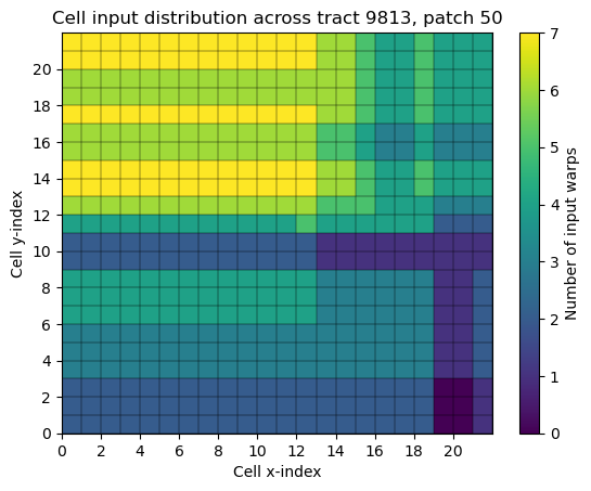
Fig. 1 A 2D histogram of the input warp distribution per cell. The gray outlines indicate the inner cell boundaries.

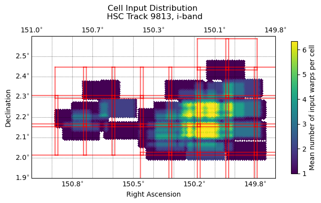
Fig. 2 Input warp distribution of 33 warps within tract 9813. Red squares represent the inner boundaries of patches, which overlap each other by two inner cell widths. These duplicate cells are removed prior to averaging values within healsparse pixels.

Cell Variance

Cell variance is one metric that can help track the quality of the cell-based coadds and shares a clear relationship with the input distribution of cells.

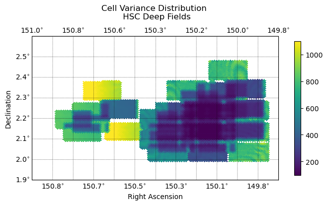
Fig. 3 The distribution of variance across cells for tract 9813. Follows the distribution of input warps closely. Variance in this case is in arbritrary flux^2 units.

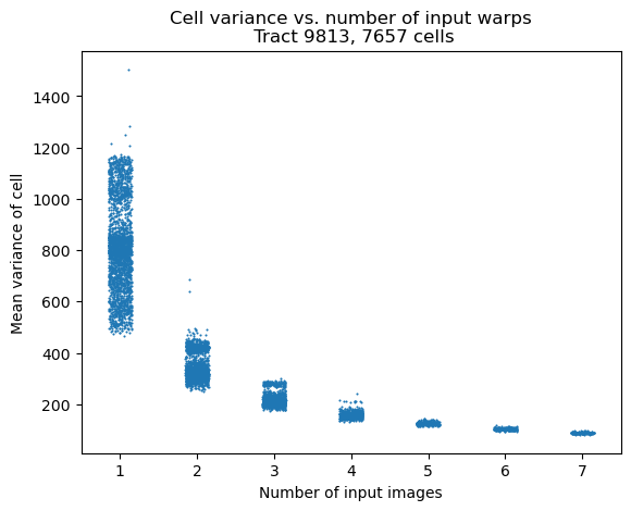
Fig. 4 Variance of a cell as a function of number of input warps. As expected, more inputs significantly improve the variance of cells. Note that each column is jittered to avoid overplotting. This reveals that the columns with 1-3 (and weakly 4) inputs have a bimodal distribution in the cell variance.

Cell Depth

Depth is another common metric to track quality of cell-based coadds. The depth definition used in this technote is the 5 sigma PSF maglim, based on the calculation done in the healsparse property maps for the pipe_tasks repo (line found here). The current zeropoint is hard-coded at 27 within the pipelines, sigma is generally set to 5. The can be written is a loose equation form:

\[ \text{magLim}=\text{zeropoint}-2.5\log_{10}\left(\text{sigma}\times\sqrt{\frac{\text{psfArea}}{\text{totalWeights}}}\right) \]

The effective PSF area is defined with:

\[ A_{\text{PSF}}=\frac{\left(\sum_i p_i\right)^2}{\sum_i p_i^2} \]

This PSF area calculation is taken from computeExposureSummaryStats.py in pipe_tasks (line found here). Each cell contains a singe realized PSF image, while each \(p_i\) value corresponds to a pixel within the PSF image. As for the total weight, this begins with the single weight of a cell calculated with _compute_weight (described earlier), which produces a single value. This value is then assigned to all pixels within the cell, and summed for the total weight.

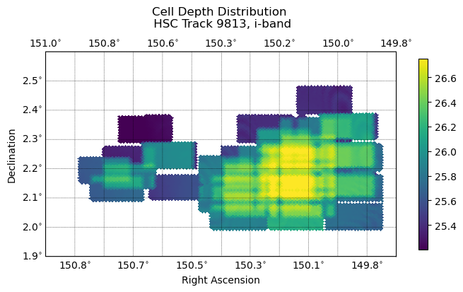
Fig. 5 The distribution of PSF maglim depth (5-sigma) across cells. Follows the distribution of input warps closely.

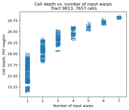
Fig. 6 Depth of a cell is calculated using PSF maglim (5-sigma). Depth increases as a function of number of inputs images. Note that each column is jittered to avoid overplotting.

Mask Fractions

The following plots are some initial analyses involving the mask fraction in cell-based coadds, though there’s still quite a bit to investigate. Figure 7 is meant to illustrate some concepts when looking at mask fractions. When tracking a bright star found in the lower right stitched coadd image, a higher mask fraction is found in the coadded mask fraction plot in the same spot, due to the interpolated bleed trails of the star. Similarly, a long track of bad columns in row 4 in the coadded mask fraction plot is also shown clearly, particularly in areas with fewer input warps.

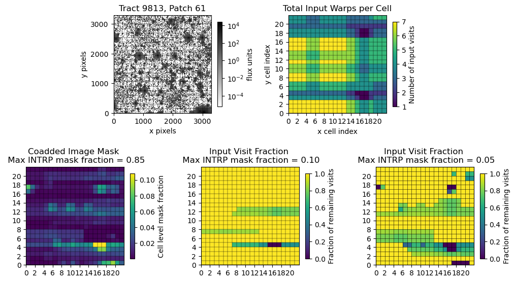
Fig. 7 Upper left: A stitched coadd image. Upper right: Inputs warps per cell Lower left: Coadded mask fraction per cell. Lower Middle: Input warp fraction of each cell, maximum threshold for warps is 10%. Lower Right: Input warp fraction of each cell, maximum threshold for warps is 5%.

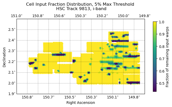
Fig. 8 The distribution of remaining input warp fraction of cells across tract 9813, at a maximum mask fraction threshold for warps at 5%; warps with a mask fraction above the threshold are discarded. Linear pattern of discarded warps likely due to column orientation, leading to patterns in bright star bleed trails, bad columns, etc.

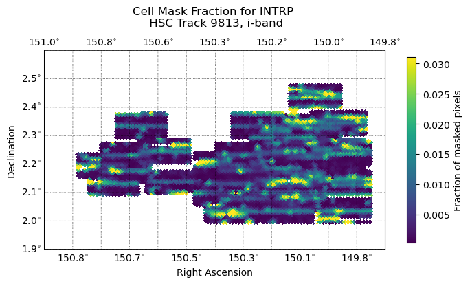
Fig. 9 The distribution of coadded mask fraction of cells across tract 9813. The maximum mask fraction threshold for warps is set to 5%; warps with a mask fraction above the threshold are discarded and not included in the coadded mask fraction. Linear pattern of discarded warps likely due to column orientation, leading to patterns in bright star bleed trails, bad columns, etc.

Maximum Mask Fraction Threshold Function

A useful metric when examining the mask fraction of coadds is the input warp fraction, which is meant to help understand how many warps are tossed when a maximum mask fraction threshold is implemented. A maximum mask fraction threshold defines the maximum mask fraction a warp can have before it is discarded from the coadd. The input warp fraction is then defined here as the remaining fraction of input warps out of the total possible after discarding warps that go over the mask fraction threshold. The total possible number of input warps includes all warps that fully cover the area of a cell, and have finite weights. A summary of this metric is seen in the maximum mask fraction threshold function. This function aims to represent the average input warp fraction of all cells in a sample for a range of maximum mask fraction thresholds.

A reasonable expectation is that as the threshold is lowered, fewer warps will remain. This appears to be the case, except for an interesting “divot” feature that is fairly consistent at a threshold of 0.016. Figure 11 narrows down the specific mask causing this divot to the BAD mask, leading to detector features as the likely cause. Figure 12 shows that this feature also appears at the patch scale, provided there are enough cells that have input warps.

The data for this section was run on w_2024_34 for tracts 9615 and 9697, and d_2024_08_24 for tract 9813.

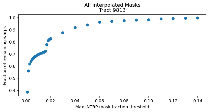
Fig. 10 The fraction of remaining input warps as a function of the maximum mask fraction threshold. Each dot is the average fraction for 7657 cells within the tract. Warps are typically only discarded once the threshold is ~15% or lower, and only noticeable closer to 10%. As expected, the number of remaining input warps per cell decreases the the threshold is lowered; this will only include input warps with very few masked pixels. Note the divot feature around 2%.

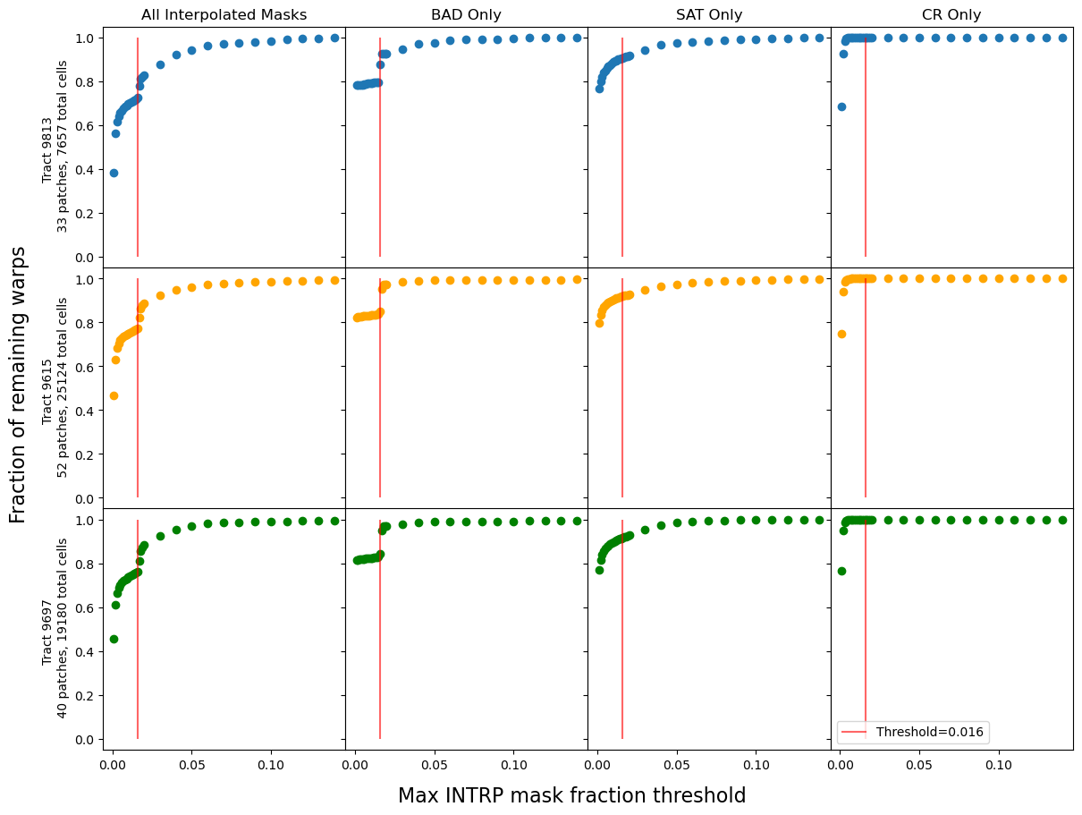
Fig. 11 Maximum mask fraction threshold functions for three tracts: 9813, 9615, and 9697. For each tract, the threshold function was generated when all three interpolated masks were included, as isolating each mask to be interpolated individually.

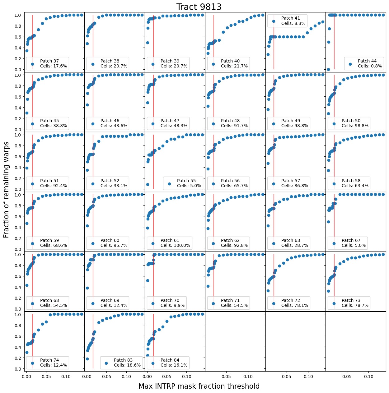
Fig. 12 Maximum mask fraction threshold functions each of the 33 patches within tract 9813. The vertical red line is placed at 0.016, which is the same reference to where the divot occurs within tract level mask fraction threshold functions. The percentage of cells indicates how many of the 484 (22 x 22) cells have input warps, indicating the statisical strength of each patch. The divot feature is most prominant in patches with most of the cell containing input warps.